What's Curved Membrane Builder Tool

Membrane curvature is a critical physical property of biological membranes, playing a fundamental role in regulating a variety of essential cellular processes, including endocytosis, exocytosis, vesicle formation, membrane fusion, and cytokinesis. In these processes, membrane curvature is not merely a byproduct of dynamic membrane remodeling but also a key driving force underlying membrane reshaping and associated molecular behaviors. Molecular dynamics (MD) simulations represent a powerful and widely utilized computational approach for investigating the interactions between membrane curvature and membrane proteins. Curved Membrane (Cmem) Builder is a versatile tool specifically designed to construct coarse-grained (CG) MD initial configurations for lipid membranes with defined curvatures and associated protein-membrane complexes. Cmem Builder offers an intuitive user interface, advanced visualization features, and extensive customization options, enabling researchers to efficiently generate curved membrane systems through automated workflows. 
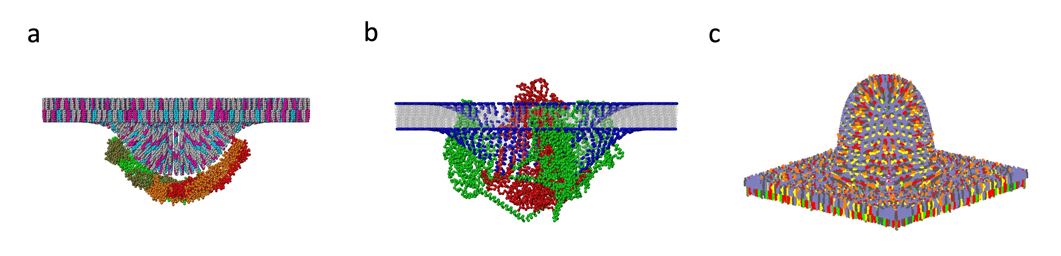
Figure 1 shows an application example of the Cmem Builder tool for constructing a curved membrane.
2
Figure 1. Curved membrane systems constructed using Cmem Builder (a) Simulation of the BAR domain embedded in a symmetric bilayer system. (b) The Piezo1 protein embedded in a curved POPC bilayer (c) Simulation of an asymmetric plasma membrane system with distinct lipid compositions in the upper and lower leaflets.

Contact us

Centre for Artificial Intelligence Driven Drug Discovery, Faculty of Applied Sciences, Macao Polytechnic University, Macao SAR 999078, China. Email:shuli@mpu.edu.mo

Tutorials

Curved Membrane Builder Tutorial

This tutorial provides a guide on how to construct a curved coarse-grained membrane system using the cmem builder. Depending on the research requirements, different Martini models can be selected, and a membrane system with curvature can be built based on PPM reference surfaces. ## 1. Selecting the Martini Model The following Martini models are available. Choose the appropriate version based on your research needs: - **Martini 2**[1] - **ELNEDYN 2**[2] - **Martini 3**[3] - **ELNEDYN 3**[2,3]
4
If only a membrane system is needed without protein involvement, select the **Non PDB** option to bypass PDB upload and directly customize the membrane curve in the drawing board. ------ ## 2. Constructing a Membrane System Using PPM Reference Surfaces If you need to build a **Membrane Only** system based on PPM reference surfaces, select **PDB options**. This includes two choices: 1. Download from OPM[4] - Directly download a PDB file with precomputed curvature from PPM. 2. Upload from PPM 3.0[5] - Upload a PDB file with membrane curvature calculated using PPM 3.0. The tool will automatically generate a reference curve based on the PPM reference curvature, ensuring that the membrane protein's position in the membrane is consistent with PPM calculations. Additionally, users can adjust control points to optimize the membrane curvature as needed. **Example:** Using PDB ID **1XQ8**, the system automatically generates reference control points and displays the reference curve in the drawing board.
10
For complex membrane surfaces, if **cubic Bézier curves** cannot accurately fit the curvature, additional **control points** can be added to improve the fit. ------ ## 3. Performing Martini Coarse-Graining The system will use **martinize2**[6] for protein coarse-graining, with results provided on the front-end. ------ ## 4. Selecting Lipid Composition In this step, you can choose the lipid composition of the **outer layer** and **inner layer** of the membrane: 1. Select the **Category** and then choose the specific **Lipid**[7]. 2. Enter the proportion for each lipid. 3. Click **Add Lipid Layer** to confirm the addition. 4. If a lipid is added incorrectly, click **Delete** to remove it.
7
------ ## 5. Adjusting Membrane Parameters & Model Construction Before constructing the membrane system, the following parameters can be adjusted to optimize membrane density and structure,Please refer to the relevant papers for detailed information. 1. **Bin Area**: Controls lipid distribution density, default value is **0.6 nm²**[7]. 2. **Normal Vector Length**: Controls the length of lipid normal vectors, default value is **30 Å**. 3. **Simulation Box**: Adjust the simulation box size to accommodate different membrane dimensions.
8
------ ## 6. Selecting the Final Output Finally, users can choose between two output formats: - **Membrane Only System** - **Protein/Membrane System**
9
With this, the curved Martini coarse-grained membrane system construction process is complete! **References:** [1] Monticelli, L.; Kandasamy, S. K.; Periole, X.; Larson, R. G.; Tieleman, D. P.; Marrink, S.-J. The MARTINI Coarse-Grained Force Field: Extension to Proteins. *J. Chem. Theory Comput.* **2008**, *4* (5), 819–834. https://doi.org/10.1021/ct700324x. [2] Periole, X.; Cavalli, M.; Marrink, S.-J.; Ceruso, M. A. Combining an Elastic Network With a Coarse-Grained Molecular Force Field: Structure, Dynamics, and Intermolecular Recognition. *J. Chem. Theory Comput.* **2009**, *5* (9), 2531–2543. https://doi.org/10.1021/ct9002114. [3] Souza, P. C. T.; Alessandri, R.; Barnoud, J.; Thallmair, S.; Faustino, I.; Grünewald, F.; Patmanidis, I.; Abdizadeh, H.; Bruininks, B. M. H.; Wassenaar, T. A.; Kroon, P. C.; Melcr, J.; Nieto, V.; Corradi, V.; Khan, H. M.; Domański, J.; Javanainen, M.; Martinez-Seara, H.; Reuter, N.; Best, R. B.; Vattulainen, I.; Monticelli, L.; Periole, X.; Tieleman, D. P.; de Vries, A. H.; Marrink, S. J. Martini 3: A General Purpose Force Field for Coarse-Grained Molecular Dynamics. *Nat. Methods* **2021**, *18* (4), 382–388. https://doi.org/10.1038/s41592-021-01098-3. [4] Lomize, M. A.; Pogozheva, I. D.; Joo, H.; Mosberg, H. I.; Lomize, A. L. OPM Database and PPM Web Server: Resources for Positioning of Proteins in Membranes. *Nucleic Acids Res.* **2011**, *40* (D1), D370–D376. https://doi.org/10.1093/nar/gkr703. [5] Lomize, A. L.; Todd, S. C.; Pogozheva, I. D. Spatial Arrangement of Proteins in Planar and Curved Membranes by PPM 3.0. *Protein Sci.* **2022**, *31* (1), 209–220. https://doi.org/10.1002/pro.4219. [6] Kroon, P.; Grunewald, F.; Barnoud, J.; van Tilburg, M.; Souza, P.; Wassenaar, T.; Marrink, S. Martinize2 and Vermouth: Unified Framework for Topology Generation. **2024**. https://doi.org/10.7554/elife.90627.2. [7] Marrink, S. J.; Corradi, V.; Souza, P. C. T.; Ingólfsson, H. I.; Tieleman, D. P.; Sansom, M. S. P. Computational Modeling of Realistic Cell Membranes. *Chem. Rev.* **2019**, *119* (9), 6184–6226. https://doi.org/10.1021/acs.chemrev.8b00460.

Select Martini Model

Main Options

Select Upper Lipid Layer

Selected Upper Lipids and Ratios

    Select Lower Lipid Layer

    Selected Lower Lipids and Ratios


      Select Output

      Theory

      Workflow of Cmem Builder.

      The Cmem Builder facilitates the construction of curved membrane systems and curved membrane-protein complex systems. Its workflow, as illustrated in Figure 1, comprises three main stages: input data, curved membrane generation, and output data. Users can provide input by specifying a protein PDB ID, uploading a PDB file, or defining curved lines to shape the membrane. System parameters such as force field, box size, lipid composition, area per lipid (APL, default: 0.6 nm²), and lipid normal displacement (LND, default: 3.0 nm) further refine the lipid assembly. The process involves obtaining curved lines, sampling the curved surface to generate coordinates and normal vectors, determining membrane curvatures, and placing lipids and water molecules. The output includes either a protein/membrane complex system or a standalone curved membrane model, offering flexibility for further simulations.

      1
      Figure 1. Overview of Cmem Builder for constructing curved membrane-protein complex systems or curved membrane systems.

      Curved membrane generation.

      The core of this procedure is the precise construction of curved surface and the accurate placement of lipids and proteins to ensure biological relevance.

      Curvature Definition

      2
      Figure 2. Construction and assembly of curved membrane systems. Curvature Definition: The membrane curvature is defined using a cubic Bézier curve, with control points determining the curvature profile. Normal vectors are calculated at sampled points along the curve to guide lipid orientation. The curved surface is generated by incrementally rotating the curve to form a complete 3D structure. Lipid Placement: Lipids are iteratively placed based on geometric criteria, ensuring proper packing density, orientation, and avoidance of particle overlap. Lipids in the upper and lower leaflets are aligned according to the normal vectors of the curved surface to maintain structural integrity and biological relevance. Components Assembly: The generated 1/8 section of the curved surface is replicated and rotated symmetrically to construct the full curved membrane. Systems can include the curved membrane alone or with embedded proteins, depending on user requirements.

      As shown in Figure 2, the XZ panel curvature is defined using a cubic Bézier curve, determined by four control points (P0, P1, P2, P3). Bézier curves are parametric curves widely used in geometric modeling due to their ability to create smooth and flexible shapes. Here, P0 and P3 define the start and end points of the curve, while P1 and P2 serve as intermediate control points that influence curvature and direction. For protein-guided curvature, control points are automatically generated based on membrane insertion data (e.g., tilt angle and depth) obtained from the OPM database. These automatically generated control points provide an initial reference and can be adjusted by users through an interactive visualization interface to fine-tune the membrane shape. Alternatively, users can manually define the control points for custom curvature designs.

      The cubic Bézier curve is mathematically expressed as:

      $$ B(t) = (1-t)^3 P_0 + 3(1-t)^2 t P_1 + 3(1-t)t^2 P_2 + t^3 P_3, \quad t \in [0,1] $$

      where B(t) is the position vector of a point on the curve at parameter t, and P0, P1,P2, and P3 are the control points. The parameter t is sampled uniformly in the range [0,1] to generate points along the curve. At each sampling point, the normal vector N(t) is computed using the derivative of the Bézier curve, B^' (t), which is given by:

      $$ B'(t) = -3(1-t)^2 P_0 + 3(1-t)^2 P_1 - 6(1-t)t P_1 + 6(1-t)t P_2 - 3t^2 P_2 + 3t^2 P_3 \quad $$

      The normal vector N(t) is obtained by normalizing the perpendicular vector to B^' (t). For Bézier curve in the XZ plane, the normalized normal vector is calculated as:

      $$ N(t) = \frac{(-B_z'(t), B_x'(t))}{\|B'(t)\|} $$

      where \(-B_z'(t)\) and \(B_x'(t)\) are the X and Z components of \(B'(t)\), and \(\|B'(t)\|\) is the magnitude of the derivative vector. These normal vectors guide the orientation of lipids during placement. The cubic Bézier equation is applied to fit the curve, generating sampling points along its length. At each sampling point, the corresponding normal vector is calculated to guide lipid placement. To construct the 3D membrane, sampling points on the Bézier curve are incrementally rotated around the Z-axis up to 45°, generating new coordinates and associated normal vectors in three-dimensional space. The rotation angle for each step is determined by the arc length of the curve, ensuring uniform sampling. A 0.1 nm arc length interval is used to balance surface resolution and computational efficiency. This process generates a 1/8 section of the curved surface, which contains sufficient geometric detail to construct the membrane. By leveraging the axial symmetry of the curved membrane, only this 1/8 section is computed initially. The complete 360° membrane is then constructed by replicating and rotating the 1/8 section around the Z-axis. This approach significantly reduces computational complexity while ensuring geometric accuracy and structural consistency.

      Lipid Placement.

      The lipid placement process begins at the starting point \( P_0 (x_0, y_0, z_0) \), the first sampled point on the Bézier surface. Placement is performed iteratively along the \( X \) and \( Y \) directions, with strict geometric criteria ensuring proper lipid packing and orientation (Figure 2).

      (1) Initial sampling in the \( Y \)-direction: Sampling points within the range \( y = y_0 \pm 0.25 \) are identified as candidate positions for lipid placement.

      (2) Lipid placement along the \( X \)-direction: For each sampling point in the \( y = y_0 \pm 0.25 \), the algorithm iterates along the \( X \)-axis from \( x_0 \) to \( x_0 + (\text{box } X)/2 \). At each \( X \)-coordinate, lipid placement is evaluated based on the following three conditions.

      • Bottom distance: The distance between the bottom virtual point of the candidate lipid and those of all previously placed lipids \( d_b (i,j) \) must exceed \( \sqrt{\text{APL}} \) (\( \text{APL} = 0.6 \, \text{nm}^2 \) by default).
      • Head distance: The distance between the head virtual point of the candidate lipid and those of all previously placed lipids \( d_h (i,j) \) must also exceed \( \sqrt{\text{APL}} \).
      • Particle overlap: Using a KDTree algorithm, it is ensured that the candidate lipid does not overlap with any previously placed lipid particles.

      If all three conditions are satisfied, the lipid is placed at the sampling point, and the algorithm proceeds to the next \( X \)-coordinate.

      (3) Termination of \( X \)-direction placement: Placement along the \( X \)-axis continues until the \( X \)-coordinate reaches \( x_0 + (\text{box } X)/2 \).

      (4) Diagonal movement in \( XY \) plane: After completing lipid placement along the \( X \)-direction, the algorithm identifies a new sampling point \( S_n (x_n, y_n, z_n) \) along the \( XY \) diagonal. The same three placement criteria are applied at \( S_n \) and if satisfied, the lipid is placed. The algorithm then continues placement from \( S_n \).

      (5) Reiteration for \( Y \)-direction: The process repeats for new \( Y \) ranges \( y = y_n \pm 0.25 \), iterating over the \( X \)-direction and diagonal movements, until \( y_0 + (\text{box } Y)/2 \) is reached, completing lipid placement in the upper leaflet. For the lower leaflet, the lipid placement process is identical, except that the lipid orientation is aligned anti-parallel to the normal vectors of the sampled surface points.

      Components Assembly.

      The generated 1/8 membrane section is symmetrically replicated and rotated in 45° increments around the Z-axis to construct the full curved bilayer (Figure 2). Water molecules are added to the system to fully solvate the membrane. For protein-membrane systems, the protein’s tilt angle and insertion depth are adjusted to match the curvature profile, ensuring proper integration with functionally relevant regions, such as curvature-sensing zones or membrane deformation sites. This alignment preserves the biological relevance of protein-membrane interactions and facilitates accurate modeling of membrane-associated processes.